AI tutoring outperforms in-class active learning: a re-analysis
AI
multilevel modeling
bootstrap
Published
January 31, 2026
I recently came across this article in Nature titled AI tutoring outperforms in-class active learning: an RCT introducing a novel research-based design in an authentic educational setting by Kestin et al. The abstract states “We find that students learn significantly more in less time when using the AI tutor, compared with the in-class active learning.” The article also claims “The median learning gains for students, relative to the pre-test baseline (M=2.75, N=316), in the AI-tutored group were over double those for students in the in-class active learning group.” (emphasis mine) That’s a really large effect!
The study utilized a cross-over design: “In this study, students were divided into two groups, each experiencing two lessons, each with distinct teaching methodologies, in consecutive weeks. During, the first week, group 1 engaged with an AI-supported lesson at home while group 2 participated in an active learning lesson in class. The conditions were reversed the following week.” This seems like a solid study design.
The authors generously shared their data on GitHub as a Stata dta file. Let’s replicate their results and critique their statistical approach.
First we’ll read in the data and look at the first 6 rows. The “rid” column is a unique identifier for each student. If we sort by “rid” we see that each student appears to have two records, one for their AI supported lesson and one for their active learning lesson, which is coded in the “lect_AI” column (0 = active learning, 1 = AI supported). We also see each student took a pre-test and post-test in each condition. The other columns are for self-reported student survey responses, which I won’t look at it in this post.
The reported pre-test baseline and group size is for all students in the study (M=2.75, N=316):
list(M =median(d$pre_score), N =length(d$pre_score))
$M
[1] 2.75

$N
[1] 316
How the authors determined learning gains were more than double was to subtract the overall pre-score median from all post-test scores and then compare differences.
d$diff <- d$post_score -median(d$pre_score)aggregate(diff ~ lect_AI, data = d, median)
  lect_AI diff
1       0 0.75
2       1 1.75
The median of the AI group is “over double” the size of the in-class group.
1.75/0.75
[1] 2.333333
However it makes more sense to compare each person’s post-test score to their own pre-test score.
When we do this the median difference is more like 30% higher.
1.583333/1.208333
[1] 1.310345
The article also says: “Students in the AI group exhibited a higher median (M) post-score (M=4.5, N=142) compared to those in the in-class active learning group (M=3.5, N=174).” We can replicate these results as follows:
# in-class = 0, AI group = 1tapply(d$post_score, d$lect_AI, function(x)c(M =median(x), N =length(x)))
$`0`
    M     N
  3.5 174.0

$`1`
    M     N
  4.5 142.0
This is also about a 30% increase:
4.5/3.5
[1] 1.285714
We can properly analyze the difference in medians controlling for pre-test using quantile regression.
library(quantreg)m <-rq(post_score ~ pre_score + lect_AI, data = d)coef(summary(m))
The expected median post-score for the AI tutored group is about 0.7 points higher than the in-class group. The 95% confidence interval says the uncertainty in this estimate ranges from about 0.48 to 0.95. The intercept, 3.1, is the expected median post-score for students who had a pre-test score of 0. We can get expected post-test scores for both groups by plugging in a representative value for pre-test. This would be a good use of the overall median (2.75). This shows about a 20% increase.
pred <-predict(m, newdata =data.frame(pre_score =2.75, lect_AI =c(0,1)))pred[2]/pred[1]
       2
1.191781
This data could also be analyzed using traditional linear modeling. The data has two records per student, so it makes sense to fit a multilevel model.
             Estimate Std. Error   t value
(Intercept) 3.1077299 0.15095904 20.586576
pre_score   0.1780523 0.04824368  3.690687
lect_AI     0.6865776 0.12143289  5.653967
The results are pretty much the same. The expected mean post-score for the AI tutored group is about 0.69 points higher than the in-class group. We can estimate an approximate 95% confidence interval by adding and subtracting two standard errors to the estimate. The 95% confidence interval says the uncertainty in this estimate ranges from about 0.43 to 0.91.
0.67+2*c(-0.12, 0.12)
[1] 0.43 0.91
Again we can get expected post-test scores for both groups by plugging in a representative value for pre-test. This also predicts about a 20% increase.
pred <-predict(m2, newdata =data.frame(pre_score =2.75, lect_AI =c(0,1)),re.form =NA)pred[2]/pred[1]
       2
1.190855
We can estimate a bootstrap confidence interval on this estimate using the bootMer() function from the lmer package.
f <-function(x){ pred <-predict(x, newdata =data.frame(pre_score =2.75, lect_AI =c(0,1)),re.form =NA) pred[2]/pred[1] }bout <-bootMer(m2, FUN = f, nsim =1000, seed =4321)quantile(bout$t, probs =c(0.025, 0.975))
    2.5%    97.5%
1.116929 1.264681
The 95% confidence interval shows an improvement of about 12% to 26%.
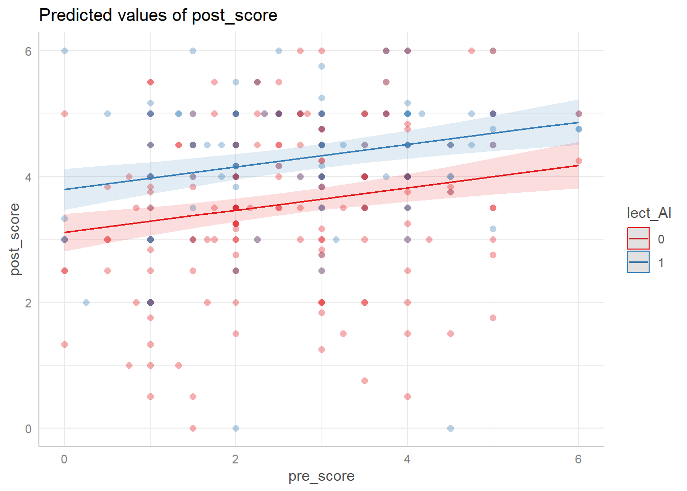
We can visualize this model using ggeffects. Notice the enormous amount of variability around the fitted lines. However, controlling for pre-score, there appears to be an expected improvement in post-scores for the AI group. The distance between the lines is the 0.69 coefficient in the model.
Yes, absolutely, the AI group seems to do better. But I wouldn’t say it doubled the effect.
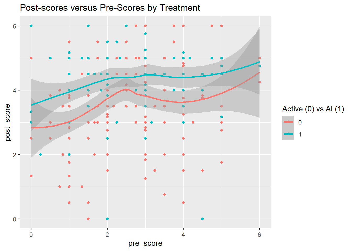
If we plot the raw data and fit nonparametric smooth trend lines, we see the same general result. Controlling for pre-score, there are slighter higher post-scores for the AI group.
library(ggplot2)ggplot(d) +aes(x = pre_score, y = post_score, color =factor(lect_AI)) +geom_point() +geom_smooth() +labs(title ="Post-scores versus Pre-Scores by Treatment", color ="Active (0) vs AI (1)")
Now if students participated in both conditions, they should have two records. But only 63% of the students participated in both conditions.
mean(table(d$rid) ==2)
[1] 0.628866
If we only analyze students in both conditions, the effect gets even smaller.
i <-names(table(d$rid))[table(d$rid) ==2]m3 <-lmer(post_score ~ pre_score + lect_AI + (1|rid), data = d, subset = d$rid %in% i)coef(summary(m3, corr =FALSE))
             Estimate Std. Error   t value
(Intercept) 3.2904147 0.16842622 19.536238
pre_score   0.1550742 0.05193203  2.986100
lect_AI     0.6100910 0.13053592  4.673741
Now the improvement is only about 16%.
pred <-predict(m3, newdata =data.frame(pre_score =2.75, lect_AI =c(0,1)),re.form =NA)pred[2]/pred[1]
       2
1.164141
Once again we can use the bootstrap to get a percentile confidence interval on this ratio.
The effect is plausibly as small as 9% or as high as 24%.
Session Details
The analysis was done using the R Statistical language (v4.5.2; R Core Team, 2025) on Windows 11 x64, using the packages lme4 (v1.1.38), Matrix (v1.7.4), SparseM (v1.84.2), quantreg (v6.1), ggeffects (v2.3.1), ggplot2 (v4.0.1) and haven (v2.5.5).
References
Douglas Bates, Martin Maechler, Ben Bolker, Steve Walker (2015). Fitting Linear Mixed-Effects Models Using lme4. Journal of Statistical Software, 67(1), 1-48. doi:10.18637/jss.v067.i01.
Kestin, G., Miller, K., Klales, A. et al. AI tutoring outperforms in-class active learning: an RCT introducing a novel research-based design in an authentic educational setting. Sci Rep 15, 17458 (2025). https://doi.org/10.1038/s41598-025-97652-6.
Lüdecke D (2018). “ggeffects: Tidy Data Frames of Marginal Effects from Regression Models.” Journal of Open Source Software, 3(26), 772. doi:10.21105/joss.00772 https://doi.org/10.21105/joss.00772.
R Core Team (2025). R: A Language and Environment for Statistical Computing. R Foundation for Statistical Computing, Vienna, Austria. https://www.R-project.org/.