The first time I took a statistics class I was mystified with z-scores. I understood how to find a z-score and look up the corresponding probability in a Standard Normal Distribution table. But I had no idea why I did it. I was just following orders. In this post I hope to explain the z-score and why it’s useful.

The first thing to understand about a z-score is that it’s simply a transformation, just like transforming inches to feet. Let’s say you and I each make our own paper airplane, throw them and measure the distance traveled. Mine flies 60 inches. Yours flies 78 inches. Yours flew 18 inches further than mine. We can transform inches to feet by multiplying by \( \frac{1}{12} \). \( 18 \times \frac{1}{12} = 1.5 \). Your airplane flew 1.5 feet further. A z-score is pretty much the same idea. You take an observation from a Normal distribution, measure how far it is from the mean of the distribution, and then convert that distance to a number of standard deviations. A quick example: I observe a measure of 67 inches from a Normal distribution with a mean of 69 and a standard deviation of 4. The z-score is calculated as \( z = \frac{67-69}{4} = -0.5\). That tells me my observation is half a standard deviation away from the mean. The negative tells me it’s less than the mean, which you knew before even doing the calculation. Also, notice there are no units. A z-score doesn’t have units like inches or kilograms. It’s just the number of standard deviations.

So that’s your z-score: distance expressed as number of standard deviations. By itself it’s kind of interesting and informative. But it’s rare you stop with the z-score. Usually in statistics the z-score is the first step toward finding a probability. For example, let’s say a candy maker produces mints that have a label weight of 20.4 grams. Assume that the distribution of the weights of these mints is Normal with a mean of 21.37 and a standard deviation of 0.4. If we select a mint at random off the production line, what is the probability it weighs more than 22.07 grams? This is a classic statistics problem. I pulled this one from Probability and Statistical Inference 7th ed. by Hogg and Tanis.

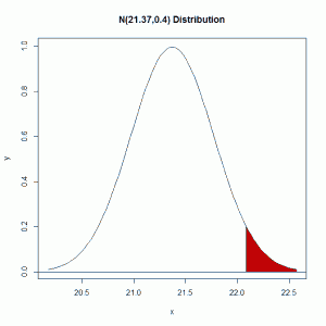
What this problem boils down to is finding the area of the red region below:

The probability of picking a piece of candy that weighs more than 22.07 grams is equal to the red area under the Normal (21.37, 0.4) distribution curve above. Nowadays this is easily done with computers and calculators. In Excel, you simply enter =1-NORMDIST(22.07,21.37,0.4,TRUE) to find the probability as 0.040059. In R, you do 1-pnorm(22.07,mean=21.37,sd=0.4). However, not so long ago, finding this area was no easy task. Mathematically speaking, finding the area means solving the following integral:

$$ \frac{1}{0.4\sqrt{2\pi}}\int_{22.07}^{\infty}exp[-(x-21.37)^2/ 2(0.4)^2] $$

Believe me when I say this is not an easy calculus problem to solve. There is no closed form solution for it. The answer has to be approximated using a power series.

Clever statisticians, however, realized that every Normal distribution can be transformed to a Standard Normal distribution using z-scores. That is, all z-scores come from a Normal distribution with mean 0 and standard deviation 1. So what they did was create a table with approximate probabilities for z-scores ranging from 0 to something like 3.49. (To see one of these tables, Google “Z-score table”). This allowed statisticians (and students) to easily solve problems like the candy problem above by transforming the value of interest to a z-score and then looking up the probability in a chart.

For our problem above, we would find \( z = \frac{22.07-21.37}{0.4} = 1.75\). Now the problem is find the probability of exceeding 1.75 in a Normal distribution with mean 0 and standard deviation 1. We would then look up 1.75 in a table and see the resulting probability. Usually the probability (or area under the curve) was calculated to the left of the z-score. For our problem we need area to the right of the z-score. If the table gave area to the left, we would simply subtract from 1. In the table I linked to, the probability for 1.75 is given as 0.9599. That’s area to the left. The area to the right is 1-0.9599 = 0.0401.

For many years, that was the TRUE value of a z-score. It allowed you to calculate areas under the normal curve by giving you a link to a table of pre-calculated values. I think most statistics classes still teach this method of finding probabilities, or at least mention it. But truth be told it’s obsolete. The math is now easily handled by computer. So while the z-score is still a useful descriptive measure of how far an observation lies from the mean of the Normal distribution from which it came, it’s no longer needed as it was in the past to find the area under the Normal curve.

So there you go, the story behind z-scores. Hopefully this post added to your understanding. If anything, I hope you appreciate what they meant to statisticians before modern computing. They truly were the only way to calculate probabilities based on a Normal distribution.