One of the first things you learn in an introductory mathematical statistics class is how to assign a probability model to the outcomes of a simple experiment. For example, say we have an urn containing the following:

• 2 blue marbles
• 3 green marbles
• 3 red marbles
• 2 yellow marbles

The experiment is to select one marble at random and note the color. Our intuition tells us to assign probabilities as follows:

• P(blue) = \( \frac{2}{10}\)
• P(green) = \( \frac{3}{10}\)
• P(red) = \( \frac{3}{10}\)
• P(yellow) = \( \frac{2}{10}\)

If we code our colors as 1=blue, 2=green, 3=red and 4=yellow, then our probability model is given by the probability mass function (p.m.f):

$$ f(1)=\frac{2}{10}, f(2)=\frac{3}{10}, f(3)=\frac{3}{10}, f(4)=\frac{2}{10} $$

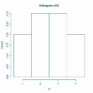
We can construct a probability histogram of this p.m.f. using R as follows:

ht <- rep(c(1,2,3,4),c(2,3,3,2))
hist(ht,freq=F,breaks=c(0.5,1.5,2.5,3.5,4.5))

This gives us the nice histogram:

If we were to actually carry out this experiment a number of times and make a histogram, we would expect to see a similar shape. This can be easily simulated on a computer. Unfortunately many textbooks don't actually tell you how to do this. Probably because doing so would mean documenting some method using some program that will likely change or be obsolete at some point. But here I show you how it can be done in R. And I can't imagine this method will go out of date any time soon.

The easy part is the simulation. One call to the rmultinom function does the trick:

rmultinom(1, 500, c(2,3,3,2))

The 1 means I'm drawing one item from the four categories containing 2, 3, 3, and 2 elements each. The 500 means I do it 500 times. The c(2,3,3,2) is a vector representing the number of colored marbles I have in each category. I also could have used the probabilities: c (0.2,0.3,0.3,0.2).

When I call this function I need to remember the results, so I give it a name, "h":

h <- rmultinom(1, 100, c(2,3,3,2))

"h" stores a matrix of numbers:

h
    [,1]
[1,] 100
[2,] 159
[3,] 141
[4,] 100

These are the results of the 500 experiments. I picked 100 blues, 159 greens, 141 reds and 100 yellows. Now to make the histogram. What I choose to do is create a vector of 500 items using the codes I assigned above (1=blue, 2=green, 3=red, and 4=yellow). I can do this using the rep() function as follows:

hx <- rep(c(1,2,3,4),c(h[1,1],h[2,1],h[3,1],h[4,1]))

The first part - c(1,2,3,4) - says I want to repeat the numbers 1, 2, 3, and 4. The second part - c(h[1,1],h[2,1],h[3,1],h[4,1]) - indicates how many times to repeat each number. h[1,1] references row 1, column 1 of the matrix called "h"; h[2,1] reference row 2, column 1 of the matrix; and so forth. Now I can use the hist function to create our histogram:

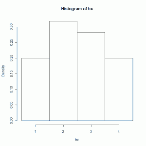
hist(hx,freq=F,breaks=c(0.5,1.5,2.5,3.5,4.5))

Here are the result:

As expected, it looks pretty close to the theoretical histogram we created first. Again, nothing mind-blowing in this post. But I did want to document one way to simulate these simple experiments we so often see early in our statistical studies.