In the final chapter the authors introduce Support Vector Machines (SVM). What SVM do are generalize linear decision boundaries for classification. Like the other chapters, this one avoids math and simply shows you how to use SVM in R. It then analyzes the spam mail dataset from chapter 3 using SVM, kNN and regularized logistic regression and compares their performance.
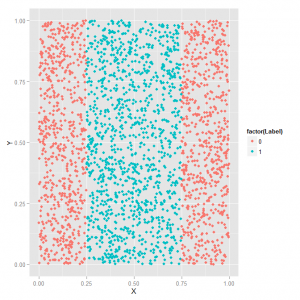
The first section of the chapter demonstrates SVM using a toy dataset. The dataset has two predictors (X and Y) and a response (a classification of 0 or 1). The dataset looks like this plotted:

I show this figure because the book is printed in black and white and you can’t tell class 0 from class 1 in the picture on page 276. That’s a problem that plagues this entire chapter. Anyway, what we have here is data that require a non-linear decision boundary. In other words we can’t draw a single straight line through the picture to indicate a boundary between the blue and red dots. This is where SVM comes in handy. Here’s the SVM code they use to analyze this dataset. As you’ll see they play around with the svm function from the e1071 package to show how changing certain parameters affects the quality of predictions. I didn’t get anything new out of this section that I felt compelled to blog about. It’s basically an extended example of how to use the svm function similar to what you might see on a help page. They do make use of the melt function from the reshape package, which is very cool and useful, but I already wrote about that in the Chapter 8 post.
The second section is “Comparing Algorithms”. They resurrect the spam dataset from chapter 3 and analyze it using SVM, kNN and regularized logistic regression. Recall the spam dataset was converted to a term document matrix (TDM) where the emails are the rows and the columns are terms. So email #1 would be row 1. In that row we would see the number of times the words in the column headers appeared. For example. the word “banner” appears 0 times in email #1. Column 1 of the spam dataset indicates whether or not the email is spam. They create testing and training sets and use those to create models and compare the different classification methods. Again, there’s nothing too fancy here where R programming is concerned, or at least nothing I haven’t already covered. They determine logistic regression works best for classifying spam email.
Now here’s something interesting worth noting. Instead of prepping the spam data as they did in Chapter 3, they skip directly to loading it into R as follows:
load('data/dtm.RData')
But how did they save that data as dtm.Rdata? By doing something like this:
save(dtm, file="dtm.RData")
…where dtm was a matrix. I say “matrix” because that’s what dtm.RData is when it gets loaded.
Another snippet worth noting is how they create their training and test sets. First they randomly select numbers as the indices for selecting the training data from the number of rows from the spam matrix. Then they take whatever numbers were not selected and make those the indices for the test data:
training.indices <- sort(sample(1:nrow(dtm), round(0.5 * nrow(dtm))))
test.indices <- which(! 1:nrow(dtm) %in% training.indices)
The dtm dataset has 3249 rows. So the sample function selects (without replacement) from the numbers 1 through 3249. The second argument to the sample function says how many to sample, which in this case is \( 0.5 \times 3249 = 1624.5 \). That gets rounded to 1624 by the round function. So 1624 numbers are sampled without replacement from the numbers 1 through 3249. And then they get sorted in ascending order. Those are the indices for the training data. To get the test data, they use the value matching %in% operator to look for matches, but negate the matches to get all the numbers that were not selected with the sample function.
The code "1:nrow(dtm) %in% training.indices" returns a logical vector with 3249 elements. 1624 are TRUE, the rest are FALSE. The code "! 1:nrow(dtm) %in% training.indices" returns the opposite logical vector. Now 1624 are FALSE and the rest are TRUE. Finally, inserting that strip of code into the which function returns the indices of the vector that are FALSE. Therefore both training.indices and test.indices are vectors of numbers from 1:3249, with no overlap between them. For example:
> training.indices[1:10]
 [1] 1 2 6 9 11 12 15 16 18 19
> test.indices[1:10]
 [1] 3 4 5 7 8 10 13 14 17 24
These vectors of numbers are then used to select the training and test data as follows:
train.x <- dtm[training.indices, 3:ncol(dtm)]
train.y <- dtm[training.indices, 1]
test.x <- dtm[test.indices, 3:ncol(dtm)]
test.y <- dtm[test.indices, 1]
I thought that was good to go through and understand since all the functions in this section require data (or are capable of taking data) in this format. For example:
library('glmnet')
regularized.logit.fit <- glmnet(train.x, train.y, family = c('binomial'))
library('e1071')
linear.svm.fit <- svm(train.x, train.y, kernel = 'linear')
library('class')
knn.fit <- knn(train.x, test.x, train.y, k = 50)
And that does it for me! I'm ready to move on to another book.