Survey a random sample of 500 men and ask if they have seen Star Wars more than twice. Survey 500 women and ask the same question. We might guess that the proportion of people in each gender who say “yes” will differ significantly. In other words, the likelihood of answering the question one way or another depends on the gender. What if we surveyed a random sample of 500 men and 500 women and asked whether or not their birthday was in December? We probably wouldn’t expect gender to influence the likelihood of having a birthday in December.

In my first example, the two variables are…

1. Have you seen Star Wars more than twice? (Yes/No)
2. Gender (Male/Female)

In the second example the two variables are…

1. Is your birthday in December? (Yes/No)
2. Gender (Male/Female)

Our question is whether or not these variables are associated.The quick way to answer this question is the chi-square test of independence. There are many good web pages that explain how to do this test and interpret the results, so I won’t re-invent the iPhone. Instead, what I want to demonstrate is why it’s called the “chi-square” test of independence.

Let’s look at the statistic for this test:

$$ \sum_{i=1}^{k}\frac{(O-E)^{2}}{E}$$

k = the number of combinations possible between the two variables. For example,

1. Male & seen Star Wars more than twice
2. Male & have not seen Star Wars more than twice
3. Female & seen Star Wars more than twice
4. Female & have not seen Star Wars more than twice

O = the OBSERVED number of occurrences for each combination. Perhaps in my survey I found 12 females out of 500 who have seen Star Wars more than twice and 488 who have not. By contrast, I found 451 males who have seen it twice and 49 who have not.

E = the EXPECTED number of occurrences IF the variables were NOT associated.

The chi-square test of independence is a hypothesis test. Therefore we make a falsifiable assumption about the two variables and calculate the probability of witnessing our data given our assumption. In this case, the falsifiable assumption is that the two variables are independent. If the two variables really are independent of one another, how likely are we to see the data we just saw? That’s a rough interpretation of the p-value.

Now let’s use R to generate a bunch of data on two independent categorical variables (each with two levels), run 1000 chi-square tests on these variables, and plot a histogram of the chi-square statistic:

p <- 0.4
n1 <- 500
n2 <- 500
n <- n1 + n2
x <- rep(NA,1000)
for (i in 1:1000){
	n11 <- sum(rbinom(n1,1,p))
	n21 <- n1 - n11
	n12 <- sum(rbinom(n2,1,p))
	n22 <- n2 - n12

	table <- matrix(c(n11,n21,n12,n22),nrow=2)
	test <- chisq.test(table,correct=F)

	x[i] <- test$statistic
	}
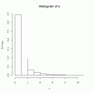
hist(x, freq=F)

>

You can see I generated two binomial samples 500 times with n=1 and p = 0.4. You can think of it as flipping a coin 500 times (or asking 500 girls if they have seen Star Wars twice). I then took the sum of the "successes" (or girls who said yes). The probabilities for both samples are the same, so they really are independent of one another. After that I calculated the chi-square test statistic using R's chisq.test function and stored it in a vector that holds a 1000 values. Finally R made us a nice histogram. As you can see, when you run the test 1000 times, you most likely will get a test statistic value below 4.

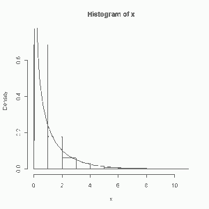
Now let's plot a chi-square distribution with one degree freedom on top of the histogram and show that the chi-square test statistic does indeed follow a chi-square distribution approximately. Note that I put approximately in italics. I really wanted you to see that. Oh, and why one degree of freedom? Because given the row and column totals in your 2 x 2 table where you store your results, you only need one cell to figure out the other three. For example, if I told you I had 1000 data points in my Star Wars study (500 men and 500 women), and that I had 650 "yes" responses to my question and 350 "no" responses, I would only need to tell you, say, that 21 women answered "yes" in order for you to figure out the other three values (men-yes, men-no, women-no). In other words, only one out of my four table cells is free to vary. Hence the one degree of freedom. Now about that histogram.

h <- hist(x, plot=F)
ylim <- range(0, h$density, 0.75)
hist(x, freq=F, ylim=ylim)
curve(dchisq(x,df=1), add = TRUE)

When I said it was approximate, I wasn't kidding was I? Below 1 the fit isn't very good. Above 2 it gets much better. Overall though it's not bad. It's approximate, and that's often good enough. Hopefully this helps you visually see where this test statistic gets its name. Often this test gets taught in a class or presented in a textbook with no visual aids whatsoever. The emphasis is on the tables and the math. But here I wanted to crawl under the hood and show you how the chi-square distribution comes into play.