Randomly select several values, say 10, from a standard Normal distribution. That’s a Normal distribution with a mean of 0 and standard deviation of 1. Now square each value and sum them all up. That sum is an observation from a chi-square distribution with 10 degrees of freedom. If you picked 12 values and did the same, you would have an observation from a chi-square distribution with 12 degrees of freedom.
We can do this in R as follows:
# random sample of 10 values from N(0,1) summed up
s <- rnorm(10)
sum(s^2)
When I did it, I got the following:
s <- rnorm(10)
s
[1] 2.3235602  0.1339985  0.5645995  1.3603184 -1.1383273  0.1735691
[7] 0.9075259  0.2842374 -0.4214184 -0.1069466
s^2
[1] 5.39893181 0.01795559 0.31877258 1.85046616 1.29578902 0.03012623
[7] 0.82360328 0.08079092 0.17759345 0.01143758
sum(s^2)
[1] 10.00547
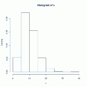
Now let's repeat this 1000 times and make a histogram:
x <- rep(NA, 1000)
for (j in 1:1000){
x[j] <-sum(rnorm(10)^2)}
hist(x)
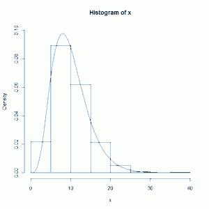
You can click on the image to see bigger version. Obviously we don't see the Normal-looking bell-shape. It skews right. Also notice that since we squared all our values, every sum is positive, which means the histogram starts at 0. Now let's plot a chi-square curve with 10 degrees of freedom on top of our histogram:
h <- hist(x, plot=F)
ylim  <- range(0, h$density, 0.10)
hist(x, freq=F, ylim=ylim)
curve(dchisq(x,df=10), add = TRUE)
I had to experiment a little to get the 0.10 value for the range statement. That was necessary to do in order to keep R from setting the displayed range of the y axis from being too small.
The formula for the chi-square curve (i.e., the probability density function) is
$$ f(x)=\frac{1}{\Gamma(r/2)2^{r/2}}x^{r/2-1}e^{-x/2}$$
where r is degrees of freedom and x must be positive. And, yes, I think it looks pretty frightening if you're not used to that sort of thing.

