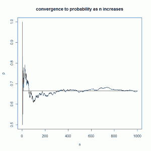
One of my favorite simulations is seeing how the relative frequency of an event stabilizes around a theoretical probability as the number of trials increases. For example, we say the probability of rolling a 5 when rolling a single die is \( \frac{1}{6}\). Although it’s an obvious probability, it’s still fun to simulate 10,000 rolls of a die and see that indeed the relative frequency of the occurrence of 5’s stabilizes around \( \frac{1}{6}\). When this concept is presented in a textbook it is often accompanied by a squiggly line graph that settles down around a straight line that represents the theoretical probability. That’s what I want to show how to do in this post, except using a dice example that does not have an obvious probability.
Let’s say we roll a single fair Las Vegas die six times and define success as follows:
- if the number on the die matches the number of the roll at least once, we have success. (So if it’s our second roll and we roll a 2, we have success.)
- If we go all six rolls with no result matching the order of the roll, we have failure.
While each roll of the die in 6 tries has a probability of \( \frac{1}{6}\) of matching the attempt number, there is no intuition for determining the probability of success as we defined it above. Theoretically we can calculate it easily enough. We note the probability of NOT rolling the same die value as attempt number is \( \frac{5}{6}\). Furthermore, the probability of NOT rolling the same die value as attempt number for all six tries is \( (\frac{5}{6})^{6}\). Now if we subtract \( (\frac{5}{6})^{6}\) from 1, we have the probability of rolling the same die value as attempt number at least once. So our probability is \( 1-(\frac{5}{6})^{6}=0.665102\). That’s pretty high. Even though success on a single roll has probability of \( \frac{1}{6}\), the probability we get at least one success in 6 rolls is about \( \frac{2}{3}\). The idea that we have a better than even chance of seeing a success in 6 rolls may be intuitive, but the theoretical probability of 0.665012 is certainly not intuitive.
We can simulate this experiment many times using a computer and check whether or not the relative frequency of success converges to the theoretical probability we calculated. We can then make one of those cool line graphs and see if the relative frequency settles down around 0.665. Here’s how I did it in R:
p <- rep(NA,1000)
s <- rep(NA,1000)
    for (j in 1:1000){
        ex <- rbinom(1,6,(1/6)) #run the experiment
        s[j] <- ifelse(ex>=1,1,0) #success or failure?
        p[j] <- sum(s,na.rm = TRUE)/j
}
The first two lines create empty vectors to store the relative frequency (p) and whether or not we saw success in each trial (s). I then execute a for loop with 1000 iterations. Each time through the loop I run the experiment using the rbinom function, I check to see if I have success using the ifelse function (storing 1 if "yes" and 0 otherwise), and then calculate the relative frequency (p). Notice that the relative frequency uses information from the previous trials in each iteration. For example, I could see a sequence such as...
- roll six times, get a success: p = 1/1
- roll six times, get a success: p= 2/2
- roll six times, no success: p = 2/3
- roll six times, get a success: p = 3/4
- roll six times, get a success: p = 4/5
Each time the denominator increases and matches the trial number. The numerator is always the previous numerator plus 1 if there was a success, or plus 0 if no success.
Once you run the simulation, you can graph it with the following:
n <- 1:1000
plot(n,p,type="l",main="convergence to probability as n increases")
lines(c(1,1000),c(0.665, 0.665))
The first line creates my x-axis values. The second line makes the plot. The third line adds a horizontal line in the graph to represent the theoretical probability. Here's how my graph turned out:
Click on it to see the graph in full-size glory.

One comment